How similar are these cells really?

A UMAP invites you to read distance as similarity: cells drawn close together look alike, cells far apart look different. UMAP keeps local neighbourhoods only approximately and can place small, isolated populations between clusters arbitrarily [Chari and Pachter, 2023]. The similarity your analysis actually uses (a kNN graph, a diffusion kernel, a pseudotime distance) is a cells × cells matrix, and it can be stored in obsp with the data.

This tutorial reads such matrices one row at a time. The focused cell picks its row, and the row colours, or places, every cell. First you follow a diffusion walk from a stem cell to a monocyte; then you plot, for one plasma cell, its UMAP distance to every cell against its diffusion distance, and find the cells where the two disagree.

The results are the panels of Fig. 3 of the AnnZarro paper (Fig. 3 · Cell by cell). If you have not used AnnZarro before, A first tour: one focused cell, one focused gene introduces the focus and the controls.

What you need

• AnnZarro with bm_aging_showcase.zarr in its data directory (Showcase store). Section 1 also works on bm_aging.zarr without the path table.

• These fields:

Slot	Key	What it is	Live or precomputed
obsm	X_umap	cell axes
obsp	diffusion_walk_t5	dense 8,090 × 8,090 five-step walk, T⁵ with T the row-normalised DM_Kernel	live: the focused cell’s row
obsp	umap_distance	dense Euclidean distance on X_umap	live
obsp	diffusion_distance	dense Euclidean distance in Palantir’s multiscale diffusion space (obsm/X_diffusion, 39 components) [Setty et al., 2019]	live
obs	fig3a_path_cell, fig3a_path_step, fig3a_focus_cells	the 13 cells on the shortest diffusion path from the HSC to the monocyte, their order 0 to 12, and four labelled stops	precomputed by the paper’s figure code
obs	fig3_plasma_groups	the plasma cell’s two discordant groups (below), with colours in uns/fig3_plasma_groups_colors	precomputed for one plasma cell
obs	highres_celltype	31 cell types

• Cells: HSC HSPC_Old_1#GAAGCCCGTGGCTCTG-1, LMPP HSPC_Old_2#ACTCTCGCAAACCGGA-1, GMP HSPC_Old_3#ATTTCACTCGTAGTGT-1, monocyte Mature_Young_2#TCAATTCAGTGAGGCT-1, plasma cell Mature_Mid_1#GCCATGGAGTATGATG-1.

Every row of these matrices is 8,090 float32 values; a focus change reads one row per panel, never the whole matrix (Pairwise matrices).

1. Follow a diffusion walk from a stem cell to a monocyte

A row of the walk matrix says where a five-step random walk on the diffusion kernel, started at the focused cell, ends up. It is a similarity that respects the data’s manifold. Walking the focus along a trajectory shows how far each cell state reaches.

1. Choose bm_aging_showcase.zarr in Dataset. Set Focused Cell to HSPC_Old_1#GAAGCCCGTGGCTCTG-1 (click the box, type, Enter, Esc).

2. In the Welcome tile click Cell Plot. X-Axis obsm · X_umap · 0, Y-Axis obsm · X_umap · 1, Color obsp · diffusion_walk_t5. The third dropdown reads “Focused cell HSPC_Old_1#…”. Color Map Blues, Reverse Colormap on.

3. Click “Split Horizontally” in the tile header and choose Cell Table. In its controls, under “Available Columns” on the obs tab, tick fig3a_path_step, fig3a_focus_cells and highres_celltype, and click Apply Changes.

4. In “Advanced Search” click Add Condition and set fig3a_focus_cells · Not · not on path. The footer reads “Showing 1 to 13 of 13 entries (filtered from 8,090 total entries)”. Click the fig3a_path_step header to sort the path from 0 (the HSC) to 12 (the monocyte). Close both panels’ controls.

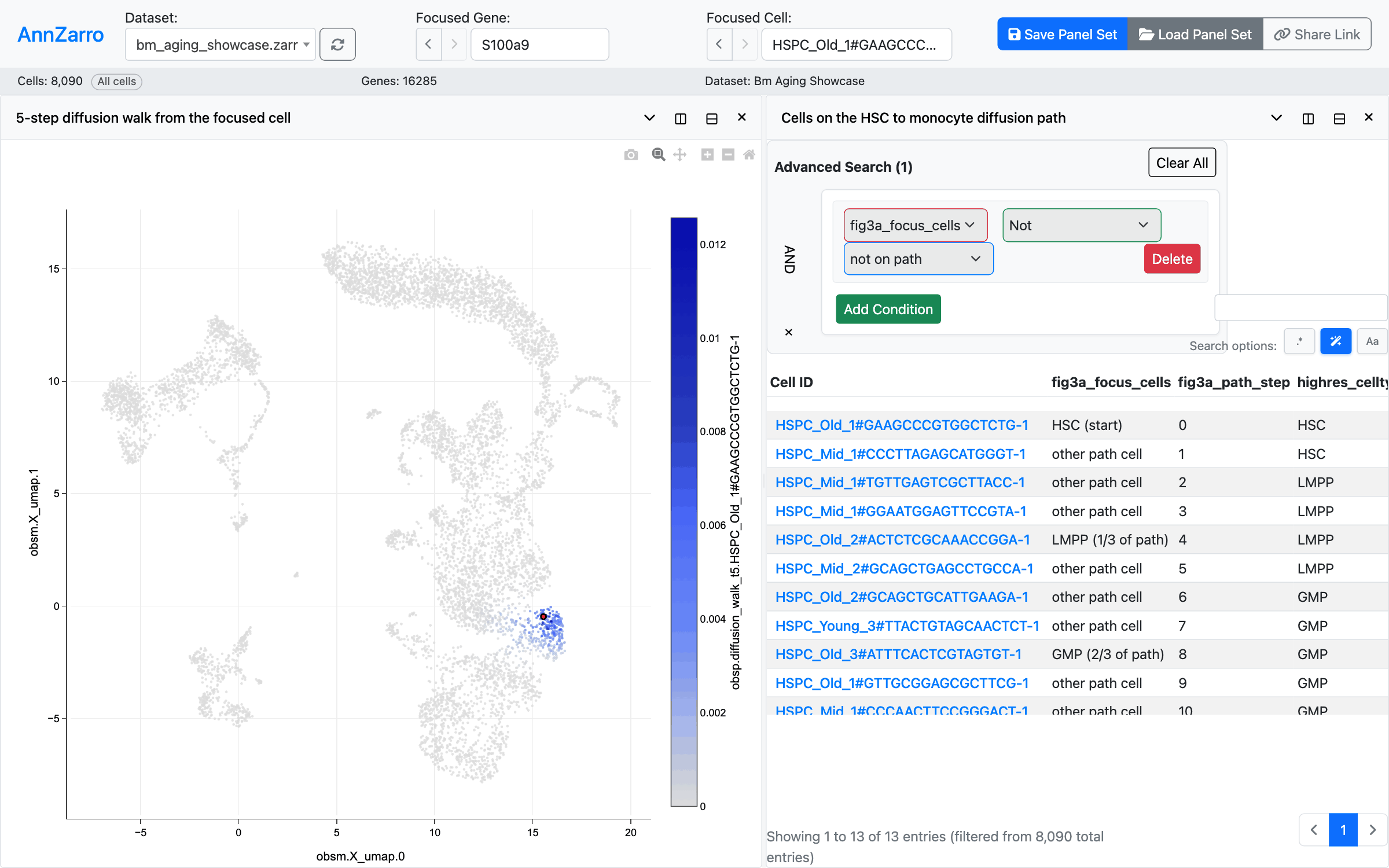
The walk from the HSC beside the 13 path cells (2 HSC, 4 LMPP, 5 GMP, 2 monocytes). The cell ID in each row is a link: clicking it focuses that cell.

5. In the table, click the cell ID in the row LMPP (1/3 of path) (HSPC_Old_2#ACTCTCGCAAACCGGA-1), then GMP (2/3 of path), then the monocyte (step 12). In a small tile the last rows sit below the visible part of the table; scroll it, or type Mature_Young_2#TCAATTCAGTGAGGCT-1 into Focused Cell.

HSC (start)

LMPP (1/3 of path)

GMP (2/3 of path)

Monocyte (end)

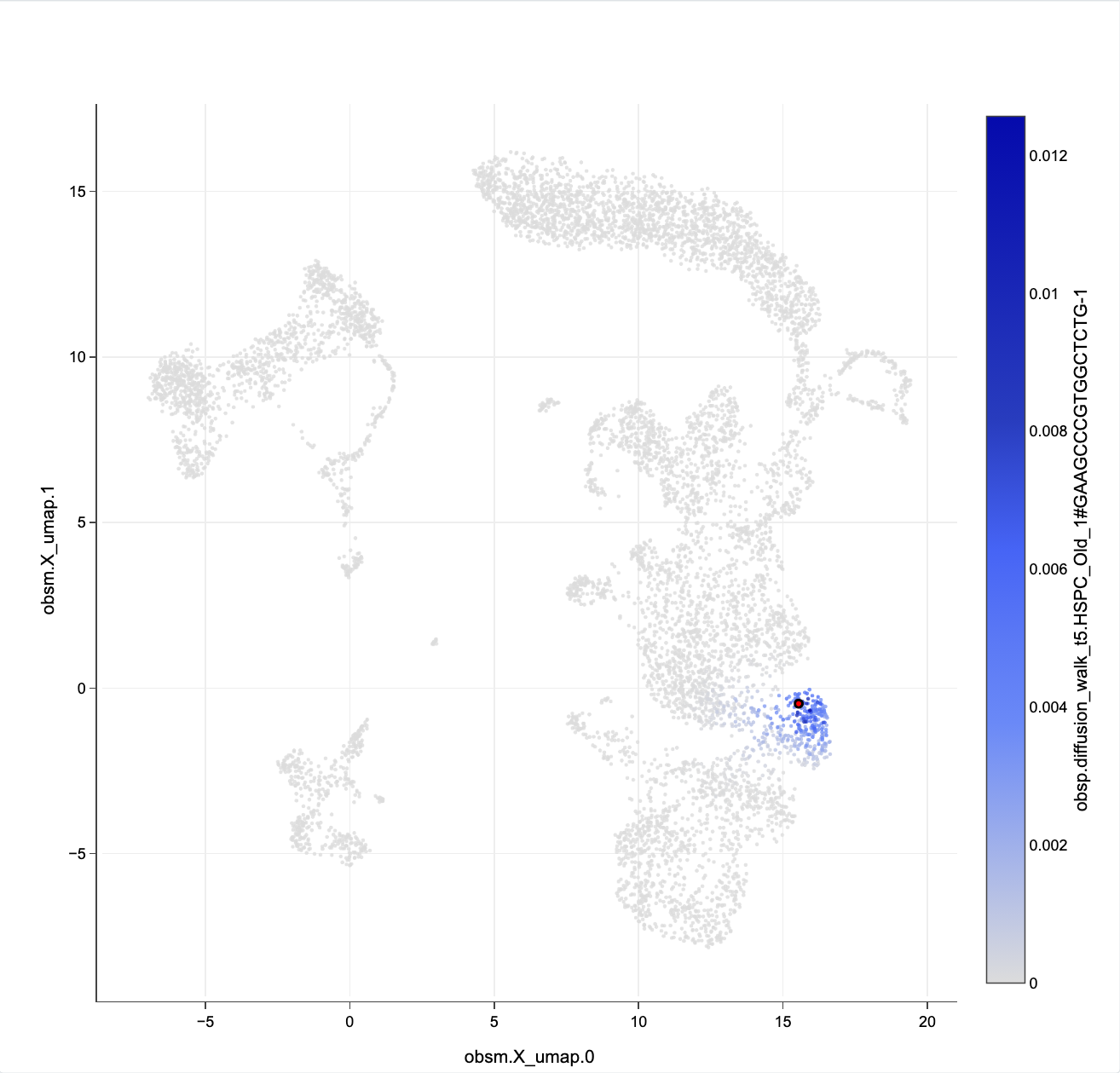
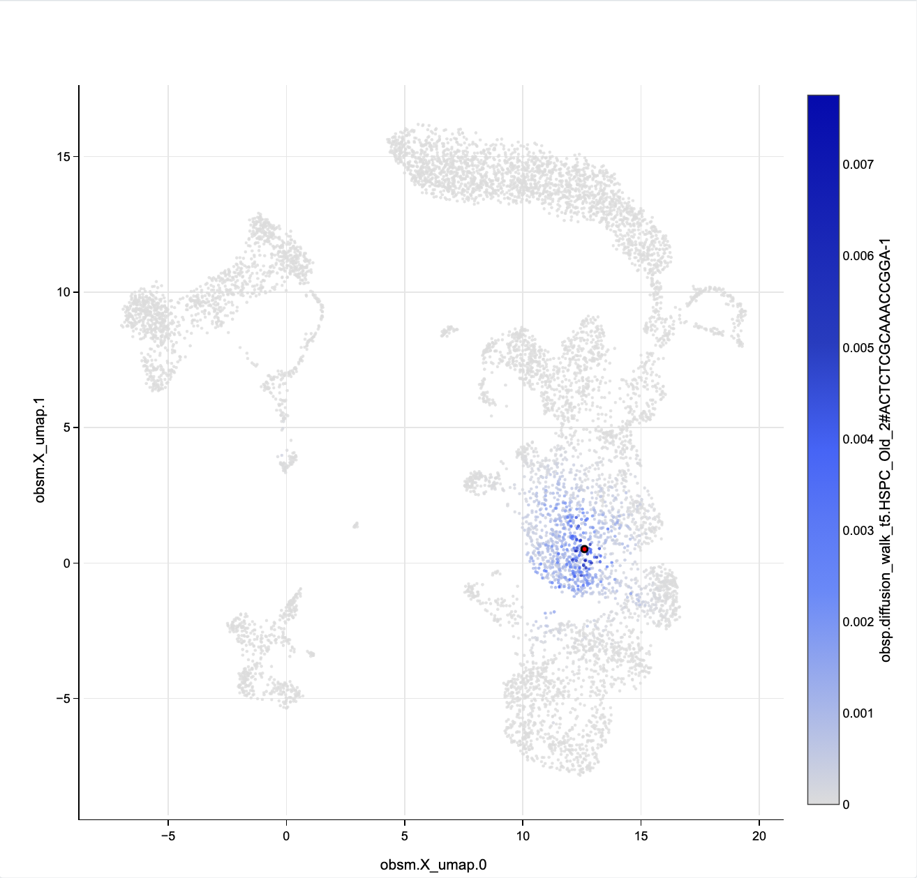
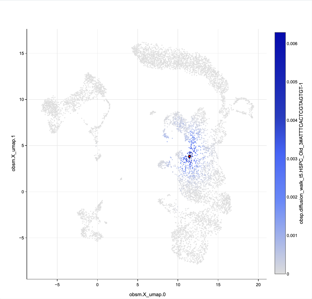
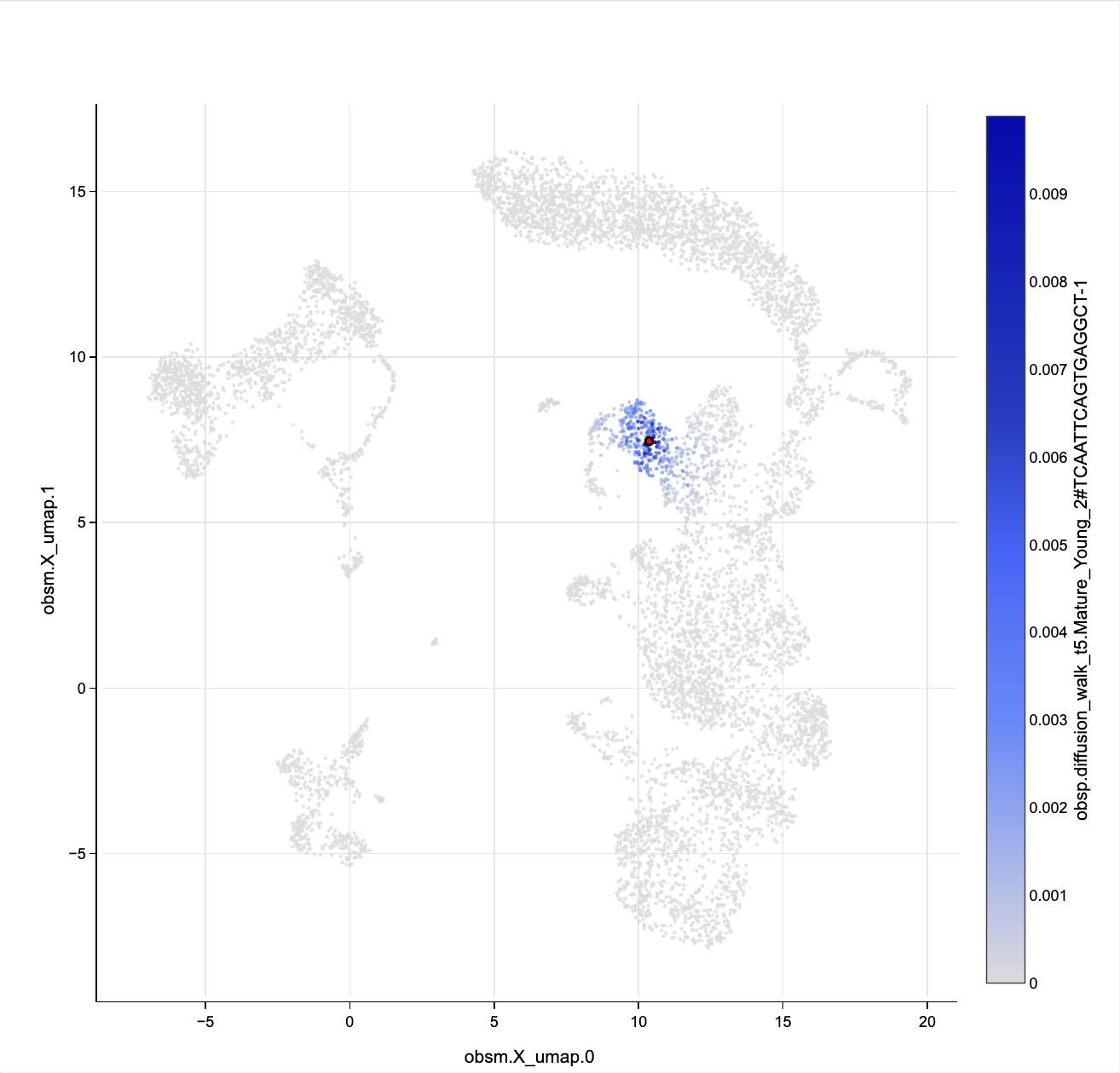
The walk spreads as it leaves the stem cell and contracts again in the monocytes. The row maxima are 0.0126 (HSC), 0.0078 (LMPP), 0.0063 (GMP) and 0.0099 (monocyte). The HSC keeps 90.7% of its walk mass among HSCs and the monocyte 88.6% among monocytes, while the GMP keeps only 24.3% among GMPs (figures/NOTES.md of the paper): a progenitor is similar to many states at once.

6. To compare the four rows on one scale, focus the HSC first, open the walk panel’s controls and click Lock Range. The colour range stays at the HSC’s, 0 to 0.0126, which is also the largest value in the four rows. Click Lock Range again to let each row scale itself.

Note

Paper Fig. 3a. The four frames are panel a of the paper figure, there drawn with a log colour scale and the path as a line (differences).

Along this trajectory the UMAP is a fair guide: the walk from each stop lands on its UMAP neighbours. The next section finds where that fails.

2. Plot UMAP distance against diffusion distance

A cell plot can take a row of obsp as an axis, not only as a colour. With the focus on one cell, each point is another cell, at x = its UMAP distance to the focus and y = its diffusion distance. Where the two agree the points fall on a rising band; where they disagree they leave it.

7. Set Focused Cell to the plasma cell Mature_Mid_1#GCCATGGAGTATGATG-1.

8. Add a Cell Plot (split a tile). Set X-Axis obsp · umap_distance and Y-Axis obsp · diffusion_distance. The third dropdown of each reads “Focused cell Mature_Mid_1#…”. Set Color obs · fig3_plasma_groups and leave Color Palette at “As stored in adata.uns if available”.

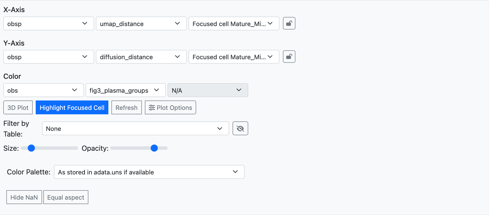
Both axes are rows of obsp that follow the focused cell. Each has its own padlock.

The colour marks two groups that the paper’s figure code computed from the plasma cell’s rank percentiles. Orange, “near in UMAP, far in diffusion”: among its 5% nearest cells on the UMAP but outside its 20% nearest in diffusion space. Blue, “far in UMAP, near in diffusion”: the reverse.

3. Find the disagreeing cells on the UMAP

9. Add a second Cell Plot with UMAP axes and Color obs · fig3_plasma_groups.

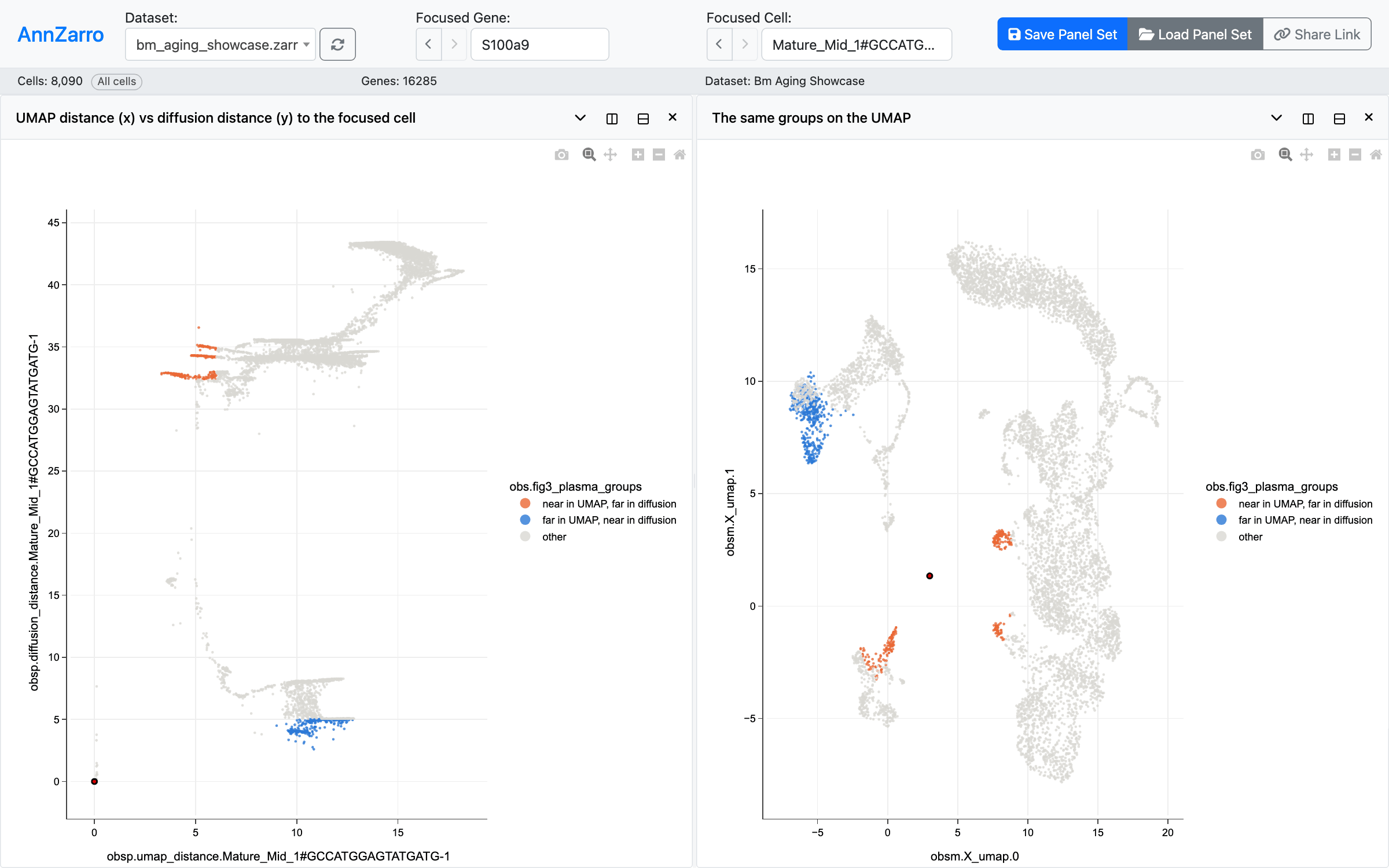
Left: orange, 265 cells, near the plasma cell on the UMAP (x from 3.3 to 6.0) but far in diffusion space (y from 32.4 to 36.6); blue, 392 cells, far on the UMAP (x from 9.0 to 12.8) but among its nearest in diffusion space (y from 2.6 to 5.0). Right: the blue cells are naive and memory B cells at the far left of the UMAP; the orange clusters sit next to the plasma cell (dark dot).

Note

Paper Fig. 3b and 3c. The two panels are panels b and c of the paper figure.

The UMAP places the plasma cell beside pDCs, NK cells, basophils and T cells, but its diffusion neighbours are B cells, its developmental relatives. In the walk matrix the orange cells receive 0.09% of the plasma cell’s walk mass and the blue cells 59.2% (paper numbers, computed offline). The plasma cells are a small population that UMAP placed between clusters; across all 8,090 cells the UMAP keeps the global rank order of diffusion distances well (median per-cell Spearman ρ 0.85) but not local neighbourhoods (median 14 of 30 nearest neighbours shared).

10. Click any other cell in the right-hand panel. The left panel redraws as that cell’s distances, because both axes follow the focus; the colours stay the plasma cell’s groups, since fig3_plasma_groups is a fixed obs column. Lock both axes (their padlocks) first to keep the plasma cell’s distances while you explore.

Check the numbers

Table filters count the groups. Add a Cell Table with the columns highres_celltype and fig3_plasma_groups and set “Advanced Search” as below. Each count was read from the app.

Statement	Advanced Search (AND)	Table footer
265 cells near in UMAP, far in diffusion	fig3_plasma_groups Equals near in UMAP, far in diffusion	265 entries
392 cells far in UMAP, near in diffusion	fig3_plasma_groups Equals far in UMAP, near in diffusion	392 entries
92 of the orange cells are pDCs, 66 NK cells	add highres_celltype Equals pDC (or NK)	92 (66) entries
274 of the blue cells are naive B cells, 111 memory B cells	add highres_celltype Equals Mature Naive B cell (or Memory B cell)	274 (111) entries
The path has 13 cells	fig3a_focus_cells Not not on path	13 entries

The Spearman ρ between the plasma cell’s two rows (0.62), the walk masses and the dataset-wide medians are not computed by AnnZarro; they come from figures/fig2_cell_by_cell.py in the paper repository and were checked when the showcase store was built (Showcase store).

Open the views

Replace /path/to/annzarro-data with the absolute path of your data directory and 127.0.0.1:8000 with your server’s address (Share links). dataset_path must be absolute.

Section 1: walk and path table

http://127.0.0.1:8000/?dataset_path=/path/to/annzarro-data/bm_aging_showcase.zarr#view=z1.jVRNb9swDP0rnnZ1hmRdgDXADqmLub2sw1ysA4bCUG3aFiJLhkRn-UD--yjZCZylxhogB5OP5CP5qD1bs8UsZJlWFrlCyxZ7VuistZBHICVbsLvke5Q-yDydvY-XyziKovgxjqPH6DGezFh4RMeggNDJbDrl12RGvtFK19v7nKxkvJ6yQ8gk3-oWXZGubiXAcJNVW7b4vWe4bVwO20iBlCIXBjIUWpGt0kbstEIuydFwBdZHNGAyIGtJcfO57wONlvansOJFkrHg0sIhPEd-Gkc-k6cSMjeghpRQECRkwjWT0VwmjdQ4eXL9j5cci0VOuMnTx_HgZ8-j8yXIEdzEzup2wPCfhMfafkIy0qoQpb2M3b_aCAp0DNh8YhGaIBdF0VqafvCHy1VQGF0HWEHQ7ztw0RS1cen6TvWLrcm0Alon-5W2NW98j7Kt3Q69ArZvx88cfscWqpXSm7U5D25OwSeyqSOb4nyY538KljpbQT4YnhYKE7GjKlf910PDM4FUafrhs1NtWUn649fhpaBpaSGVXoO5V4Ueyoe4nqimQuWwYQOBDL0utQGbuul6d6cEaj3JuF_PjWzBst74A6iadeRd9cOFHvavy-64akfcBrRit9i7JApQBzWdbbZFGAig4VidBmrHGiOtXfHUYVMnoOEGxrrtQryifMf2LUEXIzqLoXFZcE_KTUtnDKY7An8DRiAYwT1_Oq5c9G_Luy_useHIRxjR01Pedm7ikV5A0poL5abaP19ohCrpe81pVVSNKY3BcYz-tKUuRUbQ5bdbdnC_vw

Sections 2 and 3: distances as axes, groups on the UMAP

http://127.0.0.1:8000/?dataset_path=/path/to/annzarro-data/bm_aging_showcase.zarr#view=z1.3VRNi9swEP0rRr10wSl2l0LXt5BSs4fQQtJSKIvR2uNYrKwR0jjECfvfO3I-6nQ3JYeeamyM5-vNzHvyTqxFlsaiRONJGvIi24kay85DNQOtRSbmkjoHxVxVRfomn82myzyf5kt-8T1JRXyMz8EAxy_SJJF3bCa5QYNtf1-xlY13iXiOhZY9dhRg9siNAidd2fQi-7kT1NtQw1utiEtUykFJCg3bGnRqi4akZoeVBvyQYcGVwNYV531IhknIofbflVePmo211B6e46sjH9jTKF05MOOWSHFILFQYpuTNTKxGmnwK81-G_Hvu-8u5D0Mbe9-CJEFY2BnsPjA-r3dEHvajZ2hqtfIvU3evjkGKQgPi23z6NapU0EMJ0dvNTbT2_F3XnWcmRp7-JiKMqIHooIAoVORKmwBxmB0fvWXTEzDBomulLY4Fhul115qrRKaxfILq94T9JYxTp_8IaCsy02k91EB3jnoC5T3fFlZL38pi5bCzfgwadG9RGVqoLWfeHr6-WFkq4vTk3cdwEFaN5oc-j48fuY5JbnAN7t7UOFbkGL9QpoKNGGlu7A2lHfgi0DO4WV9_Kmf3qjyPmlgyyV62EO2Hi1gHgfcglZd8tyfgH0VgfLyK4R_QXx-fiv-XAr5-AQ

The same panels as panel set files (Load a panel set file): fig3-walk.json, fig3-umap-vs-diffusion.json.

Your own data

Any cells × cells matrix in obsp works the same way: a kNN graph (connectivities, distances, sparse), a diffusion kernel, Palantir or Mellon kernels, or a dense distance you compute. Dense rows are cheapest to read when each chunk holds whole rows; see Pairwise matrices for sizes and chunking. To store the two distances used here:

from scipy.spatial.distance import cdist
adata.obsp["umap_distance"] = cdist(adata.obsm["X_umap"], adata.obsm["X_umap"]).astype("float32")
adata.obsp["diffusion_distance"] = cdist(adata.obsm["X_diffusion"], adata.obsm["X_diffusion"]).astype("float32")

A dense 8,090 × 8,090 float32 matrix is 262 MB uncompressed; at a million cells a dense matrix is not practical, and a sparse kNN or kernel matrix is the better choice.

What you learned

• A row of an obsp matrix shows what one cell is similar to, by the measure you stored, not by the UMAP.

• Walking the focus along a trajectory shows how each state’s neighbourhood widens and narrows.

• Two obsp rows as axes compare two notions of distance for one cell, and the disagreeing cells can be marked and found on the UMAP.

Next: Which genes respond together? reads a genes × genes matrix the same way.