Showcase store

AnnZarro never computes anything. It shows what is stored. Some panels of the paper figures depend on numbers that the figure scripts compute in Python: the distance from one cell to all others, gene modules, the classes in a scatter. To rebuild those panels inside AnnZarro, the numbers have to be in the store.

bm_aging_showcase.zarr is Demo data (bm_aging.zarr) plus these precomputed fields. The tutorials use it (A first tour: one focused cell, one focused gene, How similar are these cells really?, Which genes respond together?, Where does a gene change, and how do two cells differ?), and so does the paper-figure appendix (Paper figures), so that every panel can be clicked through in the app. It is also a worked example of the main idea behind AnnZarro: compute once in Python, then explore without code.

• Exact copies of the paper’s analysis. Each field is computed with the code of the paper’s figure scripts, and the build script asserts the published numbers. If any one does not reproduce, the build stops.

• The original store is untouched. Its arrays are cloned unchanged. Only obs, var and the consolidated metadata are rewritten, with the new columns appended.

Added fields

Field names begin with the paper figure that uses them. General-purpose fields have plain names. The full table, with shapes, dtypes, chunking and colours, is bm_aging_showcase.FIELDS.md next to the store.

Cell x cell

Used in How similar are these cells really?; paper figure: Fig. 3 · Cell by cell.

Slot and key	What it is	Use in the app	Checked against the paper
obsp/diffusion_distance	Dense 8,090 x 8,090 Euclidean distance in Palantir’s multiscale diffusion space [Setty et al., 2019]	Focused cell’s row as a colour, or as an axis (Fig 3b)	Plasma cell row vs umap_distance row: Spearman ρ = 0.62
obsp/umap_distance	Dense Euclidean distance on X_umap	x axis of Fig 3b
obsm/X_diffusion	The multiscale diffusion space itself, 39 components: DM_EigenVectors[:, 1:40] scaled by λ/(1 − λ)	Alternative coordinates
obs/fig3_plasma_groups	The focused plasma cell’s discordant groups: near in UMAP but far in diffusion (265 cells), and the reverse (392 cells)	Colour (Fig 3b, 3c)	265 / 392 cells. Walk mass 0.09% / 59.2%.
obs/fig3_plasma_focus	The plasma cell Mature_Mid_1#GCCATGGAGTATGATG-1	Filter, or find the cell
obs/fig3_umap_dist_to_plasma, obs/fig3_diffusion_dist_to_plasma	That cell’s two distance rows as columns	Axes, where an obsp row cannot be chosen
obs/fig3a_path_cell, obs/fig3a_path_step, obs/fig3a_focus_cells	The 13 cells of the HSC to monocyte path, their order, and the four focus cells (HSC, LMPP, GMP, monocyte)	Find and focus the Fig 3a cells	Same four cells and path cell types

The kNN graph (obsp/connectivities, obsp/distances) and Palantir’s kernel were already sparse CSR matrices in the original store, so they serve as the sparse examples.

Gene x gene

Used in Which genes respond together?; paper figure: Fig. 4 · Gene by gene.

Slot and key	What it is	Use in the app	Checked against the paper
var/rho_fc_H2-Q7, var/rho_fc_H2-Aa, var/rho_fc_S100a9	That gene’s row of varp/spearman_fold_change, as a column	Gene-plot axis (the varp row itself already works as a colour)	H2-Q7’s top partners: H2-Q6 0.82, Tapbpl 0.73, H2-D1 0.66, Fxyd5 0.65, Sec62 0.63
var/rho_smoothed_H2-Q7	H2-Q7’s row of varp/spearman_smoothed	x axis of Fig 4d
var/fig4_module_k3	Average-linkage modules on 1 − ρ for the 190 DE genes, k = 3 (silhouette maximum); NA for other genes	Colour (Fig 4c)	Modules of 87, 68 and 35 genes
var/fig4c_rank_H2-Q7, var/fig4c_rank_S100a9	Rank of each DE gene by ρ with the focus gene	x axis of the ranked strips in Fig 4c	H2-Q7 in-module median ρ 0.16
var/fig4d_class	Shares the age response (fold-change ρ > 0.5), shares the cell-state pattern only (smoothed ρ > 0.7, fold-change ρ < 0.5), or other	Colour (Fig 4d)	35 and 192 genes

Cells and genes

Used in Where does a gene change, and how do two cells differ?; paper figure: Fig. 5 · Cells and genes.

Slot and key	What it is	Use in the app	Checked against the paper
layers/kompot_de_Young_to_Old_fold_change_zscores	Fold change divided by Kompot’s per-cell standard deviation, sqrt(σ²_Young + σ²_Old) [Otto et al., 2025]	Colour any gene by signal over noise; |z| > 1.96 as the noise level of Fig 5d	120 DE genes beyond 1.96 in the HSC, 13 in the monocyte. Apoe is the only opposite-direction gene beyond it in both.
var/fig5d_fc_locked_HSC, var/fig5d_fc_focused_monocyte	The two cells’ rows of the fold-change layer	Axes of Fig 5d	Apoe +0.94 / −0.35
var/fig5d_z_locked_HSC, var/fig5d_z_focused_monocyte	The same rows of the z-score layer	Filter the gene table by noise level
var/fig5d_direction	DE genes with the same or opposite sign in the two cells	Colour (Fig 5d)	129 same, 61 opposite

The z-score layer is not new to Kompot. It is the layer Kompot writes when it is run with StorageSettings(store_additional_stats=True). The demo run did not store it. The build script recomputes it from the stored fold change and per-cell standard deviations, without rerunning Kompot. A Kompot rerun with that setting confirmed the values to float32 precision.

Gene plots from varm

Slot and key	What it is	Use in the app
varm/mean_by_celltype	Mean logged_counts per gene in each of the 31 highres_celltype levels. Stored as a DataFrame whose columns are the cell-type names, in category order (also in uns/mean_by_celltype_categories).	Gene plot with one cell type per axis, e.g. HSC vs neutrophil

New categorical columns get colours in uns/<column>_colors, taken from the paper’s palette.

The showcase store and its sources look like this in the app:

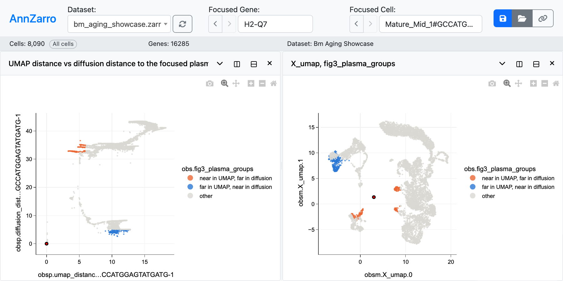
Paper Fig 3b and 3c rebuilt from the showcase store. Left: the focused plasma cell’s rows of obsp/umap_distance (x) and obsp/diffusion_distance (y), chosen as axes. Right: X_umap. Both are coloured by obs/fig3_plasma_groups with the colours stored in uns. Orange: near in UMAP, far in diffusion (265 cells). Blue: the reverse (392 cells).

Build it

The script lives in this repository’s docs folder. It reads bm_aging.zarr and imports the figure helpers of the paper repository, so it runs in the paper’s analysis environment:

cd ~/gits/annzarro            # this repository
~/gits/annzarro-paper/.venv/bin/python docs/_tools/make_showcase_store.py \
    --src ~/gits/annzarro-paper/data/bm_aging.zarr \
    --dst ~/gits/annzarro-paper/data/bm_aging_showcase.zarr

It runs in about 15 seconds on an Apple-silicon laptop. Most of that is the two 8,090² distance matrices and their ranks. The store comes to 5,739,226,831 bytes: 0.96 GB more than bm_aging.zarr. Most of that is the z-score layer (493 MB) and the two distance matrices (about 210 MB each).

The new dense arrays follow the chunk rule from Chunking:

• cells x genes chunks of (499, 1003), aspect about n_obs/n_vars at about 5 x 10⁵ values;

• obsp chunks of whole rows (62, 8090), so one focused cell’s row is one or two chunk reads.

The arrays copied from bm_aging.zarr keep their (1024, 1024) chunks.

On macOS the copy is an APFS clone, so it takes no extra space until the copy changes.

Spatial demo

The bone-marrow data have no spatial coordinates, and we do not make any up. To show spatial positions as plot axes (see Spatial coordinates), a second small store, spatial_demo.zarr, holds a public 10x Genomics Visium section of the anterior sagittal mouse brain [10x Genomics, 2020]. It is processed with scanpy [Wolf et al., 2018].

Source	10x Genomics, Mouse Brain Serial Section 1 (Sagittal-Anterior), Space Ranger 1.1.0, sample V1_Mouse_Brain_Sagittal_Anterior (dataset page)
Licence	CC BY 4.0. Reuse requires attribution to 10x Genomics.
Spots x genes	2,693 spots (of 2,695; those with ≥ 500 counts) x 2,000 highly variable genes
Size	76 MB

Processing: genes detected in ≥ 10 spots; normalised to 10⁴ counts per spot and log1p; 2,000 highly variable genes (Seurat flavour); 30 principal components; 15-nearest-neighbour graph; UMAP; Leiden clustering (resolution 0.8, 20 clusters).

Slot and key	What it holds
obsm/spatial	Spot centres in full-resolution image pixels. This is the Space Ranger convention: y grows downwards.
obsm/spatial_upright	(x, −y), so the section appears upright in a plot
obsm/X_umap, obsm/X_pca, obs/leiden	Embeddings and clusters (colours in uns/leiden_colors)
X, layers/log_normalized	Log-normalised expression, dense. The layer copy exists because AnnZarro’s plot sources list layers, not X.
layers/counts	Raw UMI counts, CSR sparse
obsp/spatial_kernel	Dense Gaussian kernel on spot distance. σ = 200 µm (two spot pitches), zero beyond 3σ, rows sum to 1. A median of 120 spots are non-zero per row.
obsp/spatial_distance	Dense spot-to-spot distance in µm. The pixel scale is calibrated on the 100 µm spot pitch.
obsp/connectivities, obsp/distances	Expression kNN graph, CSR sparse
varp/spearman_hvg	Spearman correlation of the 2,000 genes across spots, dense 2,000²
uns/source	Source URL, licence, citation and processing parameters

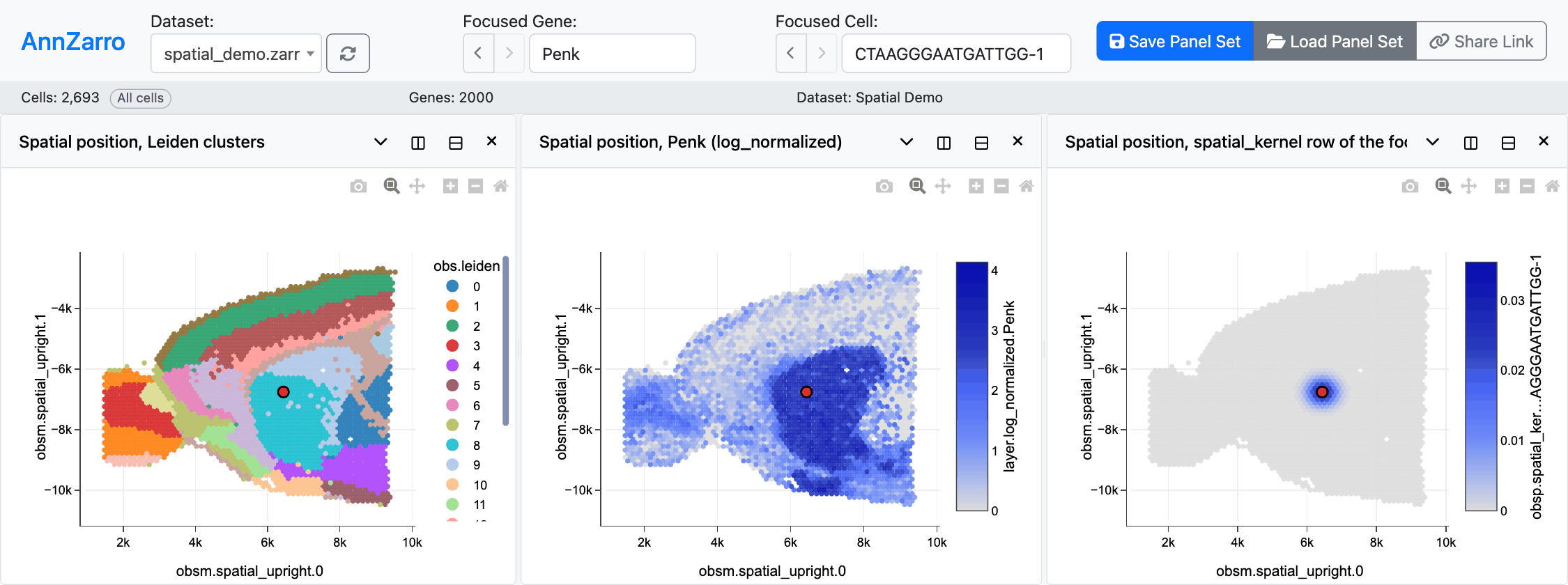
The spatial demo with obsm/spatial_upright as both axes. Left: Leiden clusters. Middle: Penk, a striatal marker, from layers/log_normalized. Right: the focused spot’s row of obsp/spatial_kernel. The focused spot is ringed in all three.

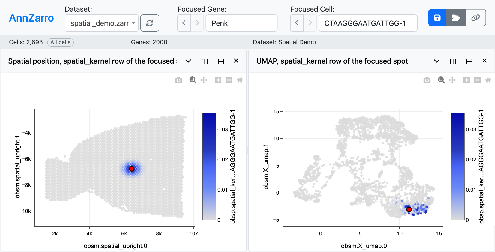
The same kernel row on the section (left) and on the expression UMAP (right). The spots around the focused spot in the tissue fall in one region of the UMAP, but not all of them next to it.

Note

Cell plots fill their tile and do not keep equal x and y scales. Spatial positions therefore stretch with the tile’s shape. Make the tile roughly square, as in these screenshots, to keep the section’s proportions.

Build it (the download is 28 MB and is cached in data/_downloads/):

~/gits/annzarro-paper/.venv/bin/python docs/_tools/make_spatial_demo.py \
    --out ~/gits/annzarro-paper/data/spatial_demo.zarr

The build takes about 10 seconds after the download.

Regenerate the screenshots

.venv-docs/bin/python docs/_tools/shoot_showcase.py --port 8813

The views are in docs/_tools/views/showcase-*.json. Each is a deep-link view object (Deep links).